You are welcome to use Jupyter Notebooks/lab as well, but note that the course will assume Rstudio and it’s best to familiarise yourself with this first.
Jupyter vs RStudio
R Console
Simplest way to interact with R
No additional features
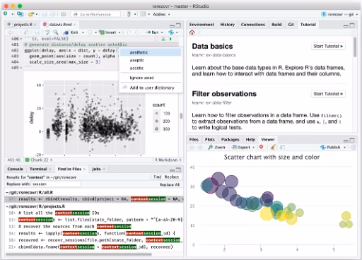
RStudio
Main IDE we will use
Includes console, scripts and much more
JupyterLab
Can use any of Julia, Python or R
Happy for you to use/try but not the focus of this course
Basic Math in R
2+2
[1] 4
5-3+2*4^2
[1] 34
11465*2358971436
[1] 27045607513740
options(scipen =999)11465*2358971436
What is the difference between these last two runs?
What do you think options(scipen = 999) is doing to the code?
options(Scipen)
‘scipen’: integer. A penalty to be applied when deciding to print numeric values in fixed or exponential notation. Positive values bias towards fixed and negative towards scientific notation: fixed notation will be preferred unless it is more than ‘scipen’ digits wider.
If I have 7 apples and 16 kids - how much of an apple do they each get?
2^16
[1] 65536
sqrt(92)
[1] 9.59166304663
7/16
[1] 0.4375
The Prompt
The prompt is represented by this symbol >.
This means that R is waiting for your input.
This is how you know that nothing is currently running.
If your code isn’t correctly formatted, R will “hang”, and you will see this symbol instead +.
You will need to kill the line to try again, and you can do this using ESC.
If this prompt is missing you know that R is running your code, depending upon the complexity of the input code this might take some time.
Try running this code in R, what happens?
5-3+2*4^
What do you think is wrong?
Commenting in R
R ignores everything after a #
You should be carefully and thoroughly commenting every bit of your code so that other people (including future you) understand what it does
It can also come after some code:
"Hello_World"# a word/character
[1] "Hello_World"
4 hashtags will also tell RStudio to allow code folding at that line, very handy for long scripts!
Getting help in R
R is great at offering extra help.
If you know the function name you can type ?function_name or help(function_name).
If you aren’t quite sure of the function name try ??function_name!
Try this out and see what you get.
?mean??meanhelp(mean)
Searching online and LLMs
Back in the not so distance past, Stackoverflow was the place to find help with codey matters…
Now most people will use Large Language Models (LLMs)
A word of caution!
They can be handy tools, but try to be very intensional about how you use them whilst learning!
You’ll be using R throughout this course, so it’s important you actually built confidence using R, not just pass the assessments
If you use them, make sure you understand the output they give you (try asking it to explain parts you don’t understand and comment any code it writes well)
Variables
We want to be able to save numbers, vectors, objects, data frames etc. so that we can call on them again later
Variable names cannot contain special characters (except _ & .), and they cannot start with a number.
<- is used to assign values to a variable
i.e. less than followed by a dash, I like to think of it as you are putting something into your variable name
Variable Assignment
x <-5y <- x +2print(y)
[1] 7
Avoid using = for assignment to avoid potential scoping issues.
Some function will only work with some data types, and some will give different types of outputs depending on the input data type, so be careful!
Type
Example
Character
‘words’
Numeric
1, 23.25
Integer
2L
Logical
TRUE, FALSE
Complex
1 + 4i
x <-3# "higher level" typeclass(x)
[1] "numeric"
# "lower level" typetypeof(x)
[1] "double"
Tables, Data Frames, Lists, Vectors
The types of data that can be stored and used in R are collectively called objects
Vectors in R
Vectors are multiple objects of the same class in one object.
We use the ‘c()’ function to join them all together.
Make your own Vector like the one below.
apple <-c('red', 'green', 'yellow')print(apple)
[1] "red" "green" "yellow"
# Check the typeprint(typeof(apple))
[1] "character"
Have a go!
Try the following:
Make two vectors of equal length, containing only numbers, save them to new variables
Add the two vectors together using their variable names, what happened?
What happens if you type name_of_your_vector[2]?
Indexing Vectors
# If we want a specific elementvec <-c("a", "b", "c", "d", "e", "f")vec[2]
[1] "b"
# If we want a range of elementsvec[3:6]
[1] "c" "d" "e" "f"
# If we want multiple specific elementsvec[c(2, 5)]
[1] "b" "e"
Vectors only contain one type of data
Vectors can only contain a single type or data, so you can’t have both characters and numerics together in one vector
What do you think happens if you try?
# What will the type of confused be?confused <-c(1, 2, "3")
print(confused)
[1] "1" "2" "3"
typeof(confused)
[1] "character"
There is an order of type conversion that R uses, with character being the broadest type
It’s common for columns you expect to be numeric to end up being characters due to a rouge value, be careful!
Operators
Relational operators
Operator
Description
<
Less than
>
Greater than
<=
Less than or equal to
>=
Greater than or equal to
==
Equal to
!=
Not equal to
Logical operators
Operator
Description
!
NOT - flips TRUE/FALSE
&
AND - TRUE if both condittions for each element
&&
AND - Same as above but for first element
|
OR - TRUE if at least one condition is TRUE for all elements
||
OR - Same as above but for first element
Operator examples
num1 <-c(TRUE, FALSE, 0, 23)num2 <-c(FALSE, FALSE, TRUE, TRUE)# Performs AND operation on each element in both num1, num2num1 & num2
[1] FALSE FALSE FALSE TRUE
# Performs OR operation on each element in both num1, num2num1 | num2
[1] TRUE FALSE TRUE TRUE
# This will convert all the num1 TRUE values to FALSE, and FALSE values to TRUE!num1
[1] FALSE TRUE TRUE FALSE
# From num2 Vector - This will convert all the TRUE values to FALSE, and FALSE to TRUE!num2
[1] TRUE TRUE FALSE FALSE
Logicals are secretly numerics
Try adding two logicals, what happens?
# What is the value of secret?secret <-TRUE+TRUE-FALSE
print(secret)
[1] 2
FALSE is actually considered to be 0 and TRUE is 1
Note that TRUE is technically any non-0 value, but normally this doesn’t matter
R is open source and easily expandable. Therefore a lot of people have contributed packages to R over the years. These are functions people have written to perform a wide variety of tasks.
There is a biology specific set of packages for R called BioConductor, and a data science one called the tidyverse (and this we will be coming back to).
You can also write your own package and submit it to the R community. We will come back to looking at packages and the writing of packages later in the course, but if you are interested there is a book about it! You can find it online here.
There are a couple of ways to install packages into R, but the easiest way is just to install them through the console and load them in like this:
Install the package.
This downloads the required code from the web repository (by default this should be “https://cran.rstudio.com/”). Packages may require other packages to work, therefore more than one package may downloaded.
install.packages('packagename')
Load the package into R.
Once the packages is downloaded, it then needs to be loaded into the R environment for use. Downloading the package does not make the commands available, it must be loaded into R first.
library(packagename)
Try installing a package!
Try and install the tidyverse and load it
Install packages from CRAN:
install.packages('tidyverse')
Load a package:
library(tidyverse)
Working Directories
Files you save have to go somewhere on your computer
R needs to know where is should save stuff
This can be done in two main ways:
Absolute paths (full system path)
Relative paths (path relative to other directories/files)
Examples:
C:/Users/matt/Dropbox/Teaching/Lesson 1 - Into to R/ - typical absolute path on Windows
03_data/my_data.csv - relative path from project root
Working Directories - continued
Use getwd() and setwd() to manage your working directory.
setwd("C:/path/to/directory")
Strongly suggest avoiding changing working directory in scripts, try to keep to relative file paths, as the absolute path is unique to your environment
If you do have absolute paths, the code won’t run on another computer and the code will break!
Check out the here package to help manage relative file paths
It helps figure out the project root based on the presence of a .Rproj file and/or a .git directory
here::here()
[1] "/Users/mateusbernardo-harrington/UK Dementia Research Institute Dropbox/Gabriel Bernardo Harrington/backup/teaching/bioinformatic_masters_r_lectures"
Importing Data
Data can be in many formats (comma separated file (.csv), Excel (.xlsx), tab delimited (.tsv or .txt))
The function you use to read in data will depend on the format of the file
# base R csv - note using here for relative paths!data <-read.csv(here::here("03_data/data.csv"))# tab and space delimiteddata <-read.table("data.tsv", sep ="\t")data <-read.table("data.txt", sep =" ")# Excellibrary(readxl) # don't forget to install the package if needed!data <-read_excel("data.xlsx", sheet =1)
Importing Data - continued
Other considerations:
Does the data have column headers
Are there leading lines to be skipped?
Is there a non-standard identifier for missing data (NA, -9, -, etc.)
What character is used as a decimal point?
How can we check the arguments we could add to these functions?
Note that there are other packages for reading in data that can be more performant, and have different default behaviour (e.g. readr or data.table)
This can be particularly important to consider when reading in larger files
Exporting Data
You’ll likely want to save the data you’ve been working with at some point
Similarly to importing data, you’ll use different functions depending on the format you want to save to
df <- mtcars # build in dataframe in R# Save to csvwrite.csv( df, here::here("03_data/mydata.csv"),row.names =FALSE,quote =FALSE)# Save to tsvwrite.table(df, here::here("03_data/mydata.tsv"), sep ="\t")
Use row.names = FALSE and quote = FALSE for better formatting.