       Name First_Name  Last_Name Age Weight Gender Married
1 Patient01    Adriana     Mattos  35   64.5      F    TRUE
5 Patient05      Janet Thomlinson  31   87.5      F   FALSE
6 Patient06 Frederique        Vos  73   69.4      F    TRUE
“A dimnames attribute for the matrix: NULL or a list of length 2 giving the row and column names respectively. An empty list is treated as NULL, and a list of length one as row names. The list can be named, and the list names will be used as names for the dimensions.”
Homework answers - continued
d <-c(1:4)e <-c("red", "white", "red", NA)f <-c(TRUE, TRUE, TRUE, FALSE)mydata <-data.frame(d, e, f)names(mydata) <-c("id", "color", "passed")mydata
  id color passed
1  1   red   TRUE
2  2 white   TRUE
3  3   red   TRUE
4  4  <NA>  FALSE
Quarto
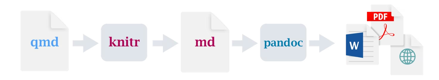
Today we’re going to talk about Quarto, which we can use to make pdf and html files (and much more!) that integrate plain language, code and output (images etc.). This is excellent because it’s a dynamic document (and so more reproducible), and hugely flexible - various languages and engines, and outputs are supported.
But before Quarto, there was Rmarkdown…
Some background on Rmarkdown
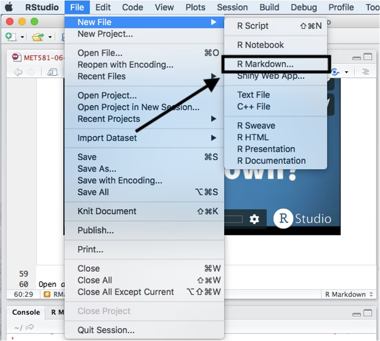
Today we will be working on a .qmd (Quarto) file, but first, we need to talk about .rmd files.
This (an .rmd file) is an Rmarkdown file. You should remember a little about markdown from your Unix lectures. You will be completing your homework in this file, so let’s have a look at it now.
RMarkdown is a way to make documents which include R code. You can use this to write html documents, pdf’s and PowerPoints to show answers to coding problems, or the code themselves.
Can you think of any reasons for using this?
Some background on Quarto
Announced in 2022 and becoming more widely adopted only last year, based on pandoc
Actually a separate software that we run within RStudio
The successor to Rmarkdown in many ways (made by the same devs), using .qmd files, made to support more languages (Python, Julia, etc.) and be more consistent in formatting
Can be used to make documents in Rstudio, or Jupyter notebooks or elsewhere (i.e. it’s both multi-language and multi-engine)
Some background on Quarto
A note on Quarto
Fundamental usage for reports is the same as creating in Rmarkdown
It’s also what’s used to make many of the R books you may read online (including R for Data Science 2nd edition!)
Recommended that you use Quarto by default, because:
You will be easily be able to swap-in other languages besides R
You will more easily be able to use other Quarto features like those for making blogs and journal articles if you’re already familiar
It’s highly compatible - you can render most Rmarkdown or jupyter notebooks in Quarto easily, so you can still make normal Rmarkdown documents with your knowledge if needed.
You’re up to date with the latest in reproducible research
Newest features will likely be added to Quarto over Rmarkdown
Making your first .qmd file
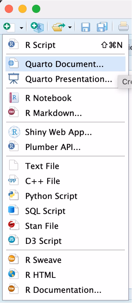
Use the menu bar to create a new Quarto document, we will focus on html today
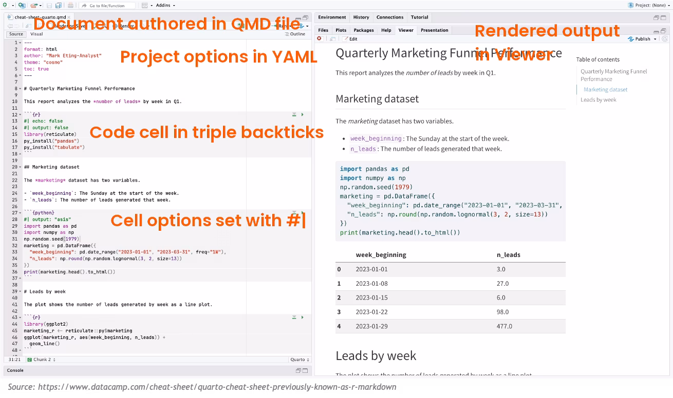
Notice that the file contains three types of content:
A YAML header surrounded by - - -
R code chunks surrounded by ```
Text mixed with simple markdown formatting
What do each of the bits of your new file do?
Let’s work through these now and create a knitted document!
Create your own with code/data you have, or download an example file from quarto from here
Elements of Quarto | The YAML header
Quarto documents start with a YAML header that sets metadata and configurations for the document.
YAML is a data serialisation language which aims to be useful for computers (often config files) and humans (it’s relatively easy to read)
Typical YAML options:
title: Title of the document
author: Author’s name
date: Document date
format: Specifies the output format (html, pdf, etc.)
theme: Defines a theme for visual style
There are a lot of options we won’t cover today and they differ by document type!
Elements of Quarto | Code chunks
When you open the file in the RStudio IDE, it becomes a notebook interface for R. You can run each code chunk by clicking the green arrow icon. RStudio executes the code and display the results in line with your file.
There are three ways to insert R code into the file:
The keyboard shortcut Ctrl + Alt + I (OS X: Cmd + Option + I)
The +option in the menu bar
Or by typing the chunk delimiters ``` {r} ```
Elements of Quarto | Code chunks
In Quarto, chunk output can be customized with options prefixed by #| inside the chunk header. Here are some common options:
#| include: false
Excludes code and results from the rendered document but runs the code.
#| echo: false
Excludes code but displays results. Useful for embedding figures.
#| message: false
Suppresses messages generated by code.
#| warning: false
Suppresses warnings generated by code.
#| fig-cap: “This is a caption”
Adds a caption to figures.
In html documents, adding code-tools and using code-folding are usually preferred over include/echo
Elements of Quarto | Inline code
Code results can be inserted directly into the text of a .qmd file by enclosing the code using single ` like so:
The mean of the data was {r} mean(mtcars$gear)
Which renders as:
The mean of the data was 3.6875
Elements of Quarto | Multiple languages
Quarto allows the use of multiple languages in code chunks. Specify the language using {} after the chunk delimiter, like python, julia, or r.
Elements of Quarto | Text Options
Do you remember your markdown formatting?
The main body is just normal markdown, so all the same stuff works
In RStudio, you can preview and render Quarto documents easily
Render by clicking the ‘Render’ button
Preview by toggling the visual button
Quarto provides a command-line interface as well, which allows rendering with: quarto render myfile.qmd
You can specify output formats in the YAML header or when rendering
Creating documents | Quarto output formats
Quarto supports various output formats:
html: Web format with dynamic features
pdf: Portable document format for printing
docx: Microsoft Word format
revealjs: HTML presentations (for slides, this is what these slide are made with!)
beamer: PDF presentations (for slides)
Specify these in the YAML or use them with the quarto render command, more details here
Creating documents | Practice
Here is a version of the document with other elements added
See if you can make an ordered list with sub items that contain at least one example of bold, italic, superscript and strikethrough text, as well as a 2x2 table with headers
Now make an .rmd file
Compare it to a .rmd document
What do you notice that’s different?
Quarto (.qmd) and Rmarkdown (.rmd): Differences you need to know
It’s pretty much mainly the syntax of the YAML options (html VS html_document), code chunk option formats (although Quarto is compatible with the rmd format), and the language support
Rmarkdown is wedded to R, even if you use other languages like Python, it’s still actually being run through R (via the reticulate package in the case of Python)
Quarto is language and engine agnostic, and thus more more versatile
“Tibbles” are a new modern data frame. It keeps many important features of the original data frame. It removes many of the outdated features. They are another amazing feature added to R by Hadley Wickham. We will use them in the tidyverse to replace the older dataframe that we just learned about.
Tibbles! - continued
Compared to Data Frames:
A tibble never changes the input type.
A tibble can have columns that are lists.
A tibble can have non-standard variable names.
can start with a number or contain spaces.
To use this refer to these in a backtick.
It only recycles vectors of length 1.
It never creates row names.
Enhanced print() behaviour
Tibbles! - continued
The syntax to make a tibble is nearly identical to data frames
library(tibble)test <-tibble(x =1:3, y =list(1:5, 1:10, 1:20))test
# A tibble: 3 × 2
      x y
  <int> <list>
1     1 <int [5]>
2     2 <int [10]>
3     3 <int [20]>
Whereas if we try this as a dataframe
test <-as.data.frame(c(x =1:3, y =list(1:5, 1:10, 1:20)))head(test)
We can easily coerce dataframes to tibbles with as_tibble()
Try the following, what differences do you notice:
data(iris)as_tibble(iris)
Tibbles on print the first 10 rows and all the columns that fit on the screen
You will not accidentally print too much!
Each column displays its data type
Tribble
Sometimes you might need to make a small table in R
tribble() allows you make a tibble and fill it row wise
The ~ is used to define column headers
tribble(~x, ~y, ~z, "a", 2, 3.6, "b", 1, 8.5)
# A tibble: 2 × 3
  x         y     z
  <chr> <dbl> <dbl>
1 a         2   3.6
2 b         1   8.5
Tibble exercises
How can you tell if an object is a tibble?
Compare and contrast the following operations on a data.frame and equivalent tibble. What is different?
df <-data.frame(abc =1, xyz ="a")df$xdf[, "xyz"]
If you have the name of a column stored in an object, e.g. var <- "mpg", how can you extract the column from a tibble?
Readr
There are many ways to import data into R, from inputting the data yourself to reading it in using the traditional R tools we used in lesson one.
The tidyverse way is to use a package called readr, there are several functions within this package you can use to read in different types of data.
Readr functions
read_csv() reads comma delimited files
read_csv2() reads semicolon separated files (common in countries where , is used as the decimal place)
read_tsv() reads tab delimited files
read_delim() reads in files with any delimiter.
read_fwf() reads fixed width files. You can specify fields either by their widths with fwf_widths() or their position with fwf_positions().
read_table() reads a common variation of fixed width files where columns are separated by white space.
read_log() reads Apache style log files.
Readr exercises
Use the base R function read.table() to import the pheno.txt file. Then repeat this with read_tsv() from Readr, what is the difference?
You may notice that read_csv automatically assumes your first row is your column headers, you may wish to alter this behaviour is your file comes with a header of information on the top row.
Open the “pheno.txt” in a text editor (can use notepad on Windows), and add a header to the file
What happens when you open this using read_csv?
Readr exercises continued
Let’s try again, but skipping this header.
You can use skip = n to skip the first n lines; or use comment = "#" to drop all lines that start with “#”
You may not have column names, in that case you can use col_names = FALSE to tell read_csv() not to treat the first row as headings, and instead label them sequentially from X1 to Xn
Readr VS base R
Why use the readr functions?
They are typically much faster (~10x) than their base equivalents. Long running jobs have a progress bar, so you can see what’s happening. If you’re looking for raw speed, try fread() from the data.table package. It doesn’t fit quite so well into the tidyverse, but it can be quite a bit faster.
They produce tibbles, they don’t convert character vectors to factors, use row names, or munge the column names. These are common sources of frustration with the base R functions.
They are more reproducible. Base R functions inherit some behaviour from your operating system and environment variables, so code that works on your computer might not work on someone else’s.